Windowed Count-Change Correct Classification Rate
Motivation: A natural metric for evaluating count-estimation performance is the Mean Absolute Error (MAE). However, using MAE to assess the count-estimation performance of an algorithm that produces counts by accumulating (summing) count changes is problematic because just a single isolated error in the count-change estimate early in time could persist forever and contribute an MAE of 1 (the so-called error-accumulation problem).
An alternative method to assess performance is to focus on count changes instead of counts. Count changes are quantitative and also discrete (integer-valued). One could focus on the quantitative aspect of count changes and evaluate performance via the MAE of count changes. An alternative approach is to ignore the numerical values of count changes and treat the discrete values, that they could possibly take, as different classes. One could then use the Correct Classification Rate (CCR) as a performance metric. However, a straightforward computation of CCR does not take into account the following important issues which arise in practice:
- Temporal mis-synchronization: the time at which the ground-truth count is deemed to change may not be matched exactly by the estimated count-change time due to subjectivity of annotators and algorithm parameters. This could substantially decrease the CCR. In practice, however, this slight temporal misalignment does not affect the occupancy estimate on a longer time scale and should be ignored.
- Sporadic and sparse count changes: ground-truth counts typically remain constant and change only occasionally. This could allow the trivial algorithm, which estimates a constant zero-valued count change, to have a very high CCR.
To address these practical problems, we propose a new CCR-like performance metric named Windowed Count-Change CCR (CCRWCC) defined below.
Definition: The new performance metric CCRWCC is described by the following equations:
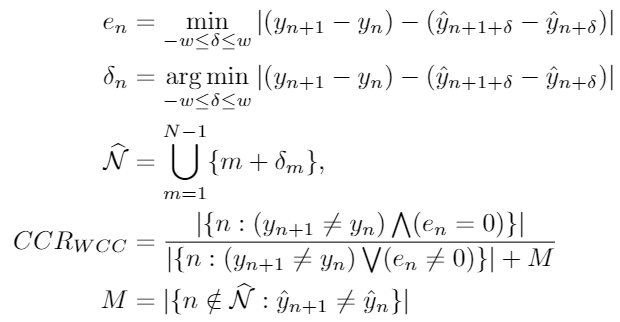
In words, the numerator of CCRWCC represents the number of count changes in the ground truth which have exactly the same count changes in the estimates within a temporal window. The denominator counts the number of time instants in which the count change in the ground truth is non-zero or the count change in the ground truth is zero, but there is no zero count change in the estimates within the temporal window. In addition, the denominator includes the number of time instants in which the count change in the estimate in non-zero, but it is not paired with any time instant in the ground truth.
Explanation: To overcome the mis-synchronization problem, for the ground-truth count change at time n , i.e., (yn+1 − yn), we find the estimated count change that best matches it within ±w time instants of time n, i.e., (ŷn+1+δn − ŷn+δn), where δn ∈ [-w, w] and n+δn is the time instant at which the estimate that best matches the ground-truth count change at time n is found. To prevent ambiguity, we adopt the convention that if δ = 0 is one of the best-matching time offsets in the range [-w, w], then δn=0. Otherwise, we set δn to be the smallest value of δ in the range [-w, w] where a best match is found. The value of w can be determined in practice via either physical constraints or by tuning it on an annotated validation dataset that is representative of the real-world environment pertinent to the application.
To prevent the small number of time instances where the count change is non-zero from being outnumbered by the much larger number of time instants where count remains constant, in CCR calculation we focus on those time instants where the ground-truth count changes, i.e., (yn+1≠yn). Additionally, we also take into account time instants where an estimated non-zero count-change is not matched to any ground-truth count change. This corresponds to the condition n ∉ N̂ in the defining equations for CCRWCC.
We now illustrate the calculation of CCRWCC through the following numerical example.
Example:
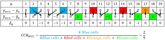
The figure shows temporal sequences of: (i) ground-truth count changes (yn+1− yn), (ii) estimated count changes (ŷn+1 − ŷn), and (iii) temporal offsets δn ∈ [-w, w], with w = 1, for which the value of (ŷn+1+δn − ŷn+δn) is closest to (yn+1 − yn). The black arrows point from time instant n in the ground-truth count-change sequence to (the best-matching) time instant n+δn in the estimate count-change sequence.
In this example, the time instants that will be contributing to the numerator are n=2 and n=6, which are the blue cells in the figure. At these two time instants, there is a non-zero count change in the ground truth which exactly equals a count change in the estimate within ±1 time instants.
In the denominator, the time instants , n = 2, 6, 10, 14 (blue and red cells) will contribute to the first term in the denominator because the count change in the ground truth at these time instants is non-zero. The time instant n = 17 (orange cell) corresponds to the situation where the count change in the ground truth is zero but there is no zero count-change in the estimate within ±1 time instants. Finally, the time instants n = 8, 12, 16, 18 (green cells) contribute to the term “M” in the defining equations, because these are the time instants which are not paired with any time instant in the ground truth during the matching process.